Binary search tree

Binary search requires an order relation by which every element (item) can be compared with every other element in the sense of a total preorder. The part of the element which effectively takes place in the comparison is called its key. Whether duplicates, i. e. different elements with the same key, shall be allowed in the tree or not, does not depend on the order relation, but on the underlying set, in other words: on the application only. For a search function supporting and handling duplicates in a tree, see section Searching with duplicates allowed.

In the context of binary search trees, a total preorder is realized most flexibly by means of a three-way comparison subroutine.

Searching in a binary search tree for a specific key can be programmed recursively or iteratively.

We begin by examining the root node. If the tree is ${\displaystyle {\text{nil}}}$, the key we are searching for does not exist in the tree. Otherwise, if the key equals that of the root, the search is successful and we return the node. If the key is less than that of the root, we search the left subtree. Similarly, if the key is greater than that of the root, we search the right subtree. This process is repeated until the key is found or the remaining subtree is ${\displaystyle {\text{nil}}}$. If the searched key is not found after a ${\displaystyle {\text{nil}}}$ subtree is reached, then the key is not present in the tree.

The following pseudocode implements the BST search procedure through recursion.[1]^: 290

 Tree-Search(x, key)
   if x = NIL or key = x.key then
     return x
   if key < x.key then
     return Tree-Search(x.left, key)
   else
     return Tree-Search(x.right, key)
   end if

The recursive version of the search can be "unrolled" into a while loop. On most machines, the iterative version is found to be more efficient.[1]^: 291

 Iterative-Tree-Search(x, key)
   while x ≠ NIL and key ≠ x.key then
     if key < x.key then
       x := x.left
     else
       x := x.right
     end if
   repeat
   return x

Since the search may proceed till some leaf node, the running time complexity of BST search is ${\displaystyle O(h)}$ where ${\displaystyle h}$ is the height of the tree. However, the worst case for BST search is ${\displaystyle O(n)}$ where ${\displaystyle n}$ is the total number of nodes in the BST, because an unbalanced BST may degenerate to a linked list. However, if the BST is height-balanced the height is ${\displaystyle O(\log n)}$.[1]^: 290

Operations such as finding a node in a BST whose key is the maximum or minimum are critical in certain operations, such as determining the successor and predecessor of nodes. Following is the pseudocode for the operations.[1]^{: 291–292}

 Tree-Maximum(x)
   while x.right ≠ NIL then
     x := x.right
   repeat
   return x

 Tree-Minimum(x)
   while x.left ≠ NIL then
     x := x.left
   repeat
   return x

For certain operations, given a node ${\displaystyle x}$, we need to find the successor or predecessor of ${\displaystyle x}$. Assuming all the keys of the BST are distinct, the successor of a node ${\displaystyle x}$ in BST is the node with the smallest key greater than ${\displaystyle x}$'s key. On the other hand, the predecessor of a node ${\displaystyle x}$ in BST is the node with the largest key smaller than ${\displaystyle x}$'s key. Following is pseudocode for finding the successor and predecessor of a node ${\displaystyle x}$ in BST.[1]^{: 292–293}

 Tree-Successor(x)
   if x.right ≠ NIL then
     return Tree-Minimum(x.right)
   end if
   y := x.parent
   while y ≠ NIL and x = y.right then
     x := y
     y := y.parent
   repeat
   return y

 Tree-Predecessor(x)
   if x.left ≠ NIL then
     return Tree-Maximum(x.left)
   end if
   y := x.parent
   while y ≠ NIL and x = y.left then
     x := y
     y := y.parent
   repeat
   return y

A BST can be traversed through three basic algorithms: inorder, preorder, and postorder tree walk.[1]^: 287

• Inorder tree walk: Nodes from the left subtree get visited first, followed by the root node and right subtree.
• Preorder tree walk: The root node gets visited first, followed by left and right subtrees.
• Postorder tree walk: Nodes from the left subtree get visited first, followed by the right subtree, and finally the root.

Following is a recursive implementation of the tree walks.[1]^{: 287–289}

 Inorder-Tree-Walk(x)
   if ≠ NIL then
     Inorder-Tree-Walk(x.left)
     visit node
     Inorder-Tree-Walk(x.right)
   end if

 Preorder-Tree-Walk(x)
   if ≠ NIL then
     visit node
     Preorder-Tree-Walk(x.left)
     Preorder-Tree-Walk(x.right)
   end if

 Postorder-Tree-Walk(x)
   if ≠ NIL then
     Postorder-Tree-Walk(x.left)
     Postorder-Tree-Walk(x.right)
     visit node
   end if

Height of the binary search tree is defined as the maximum of the heights of left subtree and right subtree incremented by a factor of 1. Following is a recursive procedure for calculating the height of the BST given a root ${\displaystyle x}$:[2]^: 303-304

 Tree-Height(x)
   if x = NIL then
     return -1
   end if
   left_height := Tree-Height(x.left)
   right_height := Tree-Height(x.right)
   if left_height > right_height then
     return left_height + 1
   else
     return right_height + 1
   end if

Operations such as insertion and deletion cause the BST representation to change dynamically. The data structure must be modified in such a way that the properties of BST continue to hold. New nodes are inserted as leaf nodes in the BST.[1]^{: 294–295} Following is an iterative implementation of the insertion operation.[1]^: 294

1    Tree-Insert(T, z)
2      y := NIL
3      x := T.root
4      while x ≠ NIL do
5        y := x
6        if z.key < x.key then
7          x := x.left
8        else
9          x := x.right
10       end if
11    repeat
12    z.parent := y
13    if y = NIL then
14      T.root := z
15    else if z.key < y.key then
16      y.left := z
17    else
18      y.right := z
19    end if

The procedure maintains a "trailing pointer" y as a parent of x. After initialization on line 2, the while loop along the lines 4-11 causes the pointers to be updated. If y is nil, the BST is empty, thus z is inserted as the root node of the binary search tree T, if it isn't nil, we compare the keys on the lines 15-19 and insert the node accordingly.[1]^: 295

Fig. 2: Binary search tree special cases deletion illustration.

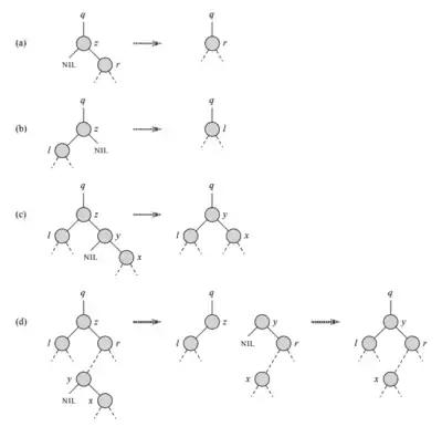
Deletion of a node ${\displaystyle {\text{z}}}$ from a binary search tree ${\displaystyle {\text{T}}}$ has three cases:[1]^: 295

1. If ${\displaystyle {\text{z}}}$ is a leaf node, we remove ${\displaystyle {\text{z}}}$ by replacing its parent with ${\displaystyle {\text{nil}}}$ as its child.
2. If ${\displaystyle {\text{z}}}$ has only one child, we elevate that child—either left or right—to ${\displaystyle {\text{z}}}$'s position by modifying ${\displaystyle {\text{z}}}$'s parent by replacing it with ${\displaystyle {\text{z}}}$'s child, as shown in fig. 2 part (a) and (b).
3. If ${\displaystyle {\text{z}}}$ has both a left and right child, we find ${\displaystyle {\text{z}}}$'s successor ${\displaystyle {\text{y}}}$ and have it take ${\displaystyle {\text{z}}}$'s position in the tree. ${\displaystyle {\text{z}}}$'s original right subtree becomes ${\displaystyle {\text{y}}}$'s new right subtree and ${\displaystyle {\text{z}}}$'s left subtree becomes ${\displaystyle {\text{y}}}$'s new left subtree respectively. However, this case isn't trivial, since it depends on the position of ${\displaystyle {\text{y}}}$ in the BST.[1]^: 296
   1. If ${\displaystyle {\text{y}}}$ is ${\displaystyle {\text{z}}}$'s right child, we elevate ${\displaystyle {\text{y}}}$ by leaving ${\displaystyle {\text{y}}}$'s right child alone, as shown in fig. 2 part (c).
   2. If ${\displaystyle {\text{y}}}$ isn't the right child, but lies within the right subtree and have a left child—either ${\displaystyle {\text{nil}}}$ or a subtree—we first replace ${\displaystyle {\text{y}}}$ by its own right child, and then replace ${\displaystyle {\text{z}}}$ with ${\displaystyle {\text{y}}}$, as shown in fig. 2 part (d).

Following is a pseudocode for the deletion operation in a binary search tree.[1]^: 296-298

1    Tree-Delete(T, z)
2      if z.left = NIL then
3        Subtree-Shift(T, z, z.right)
4      else if z.right = NIL then
5        Subtree-Shift(T, z, z.left)
6      else
7        y := Tree-Successor(z)
8        if y.parent ≠ z then
9          Subtree-Shift(T, y, y.right)
10         y.right := z.right
11         y.right.parent := y
12       end if
13       Subtree-Shift(T, z, y)
14       y.left := z.left
15       y.left.parent := y
16     end if

1    Subtree-Shift(T, u, v)
2      if u.parent = NIL then
3        T.root := v
4      else if u = u.parent.left then
5        u.parent.left := v
5      else
6        u.parent.right := v
7      end if
8      if v ≠ NIL then
9        v.parent := u.parent
10     end if

The ${\displaystyle {\text{Tree-Delete}}}$ procedure deals with the 3 special cases mentioned above. Lines 2-3 deal with case 1; lines 4-5 deal with case 2 and lines 6-16 for case 3 respectively. The helper function ${\displaystyle {\text{Tree-Shift}}}$ is used within the deletion algorithm for the purpose of replacing the node ${\displaystyle {\text{u}}}$ with ${\displaystyle {\text{v}}}$ in the binary search tree ${\displaystyle {\text{T}}}$.[1]^: 298

A binary search tree can be used in sorting algorithm implementation. The process involves inserting all the elements which are to be sorted and performing inorder traversal. This method is similar to that of quicksort where each node corresponds to a partitioning item that subdivides its descendants into smaller keys and larger keys.[3]

Binary search trees are used in implementing priority queues, using the element or node's key as priorities. Adding new elements to the queue follows the regular BST ${\displaystyle {\text{Tree-Insert}}}$ operation; but the removal operation depends on the type of priority queue:[4]

• If it's an ascending order priority queue, removal of an element with the lowest priority is done through leftward traversal of the BST i.e. ${\displaystyle {\text{Tree-Minimum }}}$.
• On the other hand, if it's a descending order priority queue, removal of an element with the highest priority is done through rightward traversal of the BST i.e. ${\displaystyle {\text{Tree-Maximum }}}$.

In regards to performance characteristics of binary search trees, a study shows that Treaps perform better on average case, while red–black tree was found to have the smallest number of performance variations.[8]

Optimal binary search tree is a theoretical computer science problem which deals with constructing an "optimal" binary search trees that enables smallest possible search time for a given sequence of accesses.[9]^{: 449–450} The computational cost required to maintain an "optimal" search tree can be justified if search is more dominant activity in the tree than insertion or deletion.[10][9]^: 449

A threaded binary search tree is an accessorial version of a binary tree whose ${\displaystyle nil}$ pointers—either left or right fields of a node—points to the inorder successor or inorder predecessor of the given nodes such that efficient utilization of the placeholders fields are performed.[2]^: 311-312 Threading is classified into two categories:[2]^: 312

• One-way threading: The left or right pointer field of the nodes, holds a reference to the inorder predecessor or inorder successor, but not both.
• Two-way threading: The left and right pointer fields hold the references to the inorder predecessor and inorder successor respectively.

References

- Cormen, Thomas H.; Leiserson, Charles E.; Rivest, Ronald L.; Stein, Clifford (2001). Introduction to Algorithms (2nd ed.). MIT Press. ISBN 0-262-03293-7.
- Thareja, Reema (13 October 2018). "Hashing and Collision". Data Structures Using C (2 ed.). Oxford University Press. ISBN 9780198099307.
- Narayanan, Arvind (2019). "COS226: Binary search trees". Princeton University School of Engineering and Applied Science. Archived from the original on 22 March 2021. Retrieved 21 October 2021 – via cs.princeton.edu.
- Myers, Andrew. "CS 2112 Lecture and Recitation Notes: Priority Queues and Heaps". Cornell University, Department of Computer Science. Archived from the original on 21 October 2021. Retrieved 21 October 2021.
- Lehman, Tobin J.; Carey, Michael J. (25–28 August 1986). A Study of Index Structures for Main Memory Database Management Systems. Twelfth International Conference on Very Large Databases (VLDB 1986). Kyoto. ISBN 0-934613-18-4.
- Demaine, E. D.; Harmon, D.; Iacono, J.; Pătraşcu, M. (2007). "Dynamic Optimality—Almost" (PDF). SIAM Journal on Computing. 37 (1): 240. doi:10.1137/S0097539705447347. S2CID 1480961. Archived (PDF) from the original on 27 February 2021 – via erikdemaine.org.
- Thornton, Alex (2021). "ICS 46: Binary Search Trees". University of California, Irvine. Archived from the original on 4 July 2021. Retrieved 21 October 2021.
- Heger, Dominique A. (2004), "A Disquisition on The Performance Behavior of Binary Search Tree Data Structures" (PDF), European Journal for the Informatics Professional, 5 (5): 67–75, archived from the original (PDF) on 2014-03-27, retrieved 2010-10-16 – via Archive.org
- Korah, A.P.; Kaimal, M.R. (1990). "Dynamic Optimal Binary Search Tree". International Journal of Foundations of Computer Science. 1 (4): 449–463. doi:10.1142/S0129054190000308 – via World Scientific.
- Gonnet, Gaston. "Optimal Binary Search Trees". Scientific Computation. ETH Zürich. Archived from the original on 12 October 2014. Retrieved 1 December 2013.
Further reading
This article incorporates public domain material from the NIST document: Black, Paul E. "Binary Search Tree". Dictionary of Algorithms and Data Structures.
- Cormen, Thomas H.; Leiserson, Charles E.; Rivest, Ronald L.; Stein, Clifford (2001). "12: Binary search trees, 15.5: Optimal binary search trees". Introduction to Algorithms (2nd ed.). MIT Press. pp. 253–272, 356–363. ISBN 0-262-03293-7.
- Jarc, Duane J. (3 December 2005). "Binary Tree Traversals". Interactive Data Structure Visualizations. University of Maryland. Archived from the original on 27 February 2014. Retrieved 30 April 2006.
- Knuth, Donald (1997). "6.2.2: Binary Tree Searching". The Art of Computer Programming. 3: "Sorting and Searching" (3rd ed.). Addison-Wesley. pp. 426–458. ISBN 0-201-89685-0.
- Long, Sean. "Binary Search Tree" (PPT). Data Structures and Algorithms Visualization-A PowerPoint Slides Based Approach. SUNY Oneonta.
- Parlante, Nick (2001). "Binary Trees". CS Education Library. Stanford University.
External links