Gauss–Legendre method

In numerical analysis and scientific computing, the Gauss–Legendre methods are a family of numerical methods for ordinary differential equations. Gauss–Legendre methods are implicit Runge–Kutta methods. More specifically, they are collocation methods based on the points of Gauss–Legendre quadrature. The Gauss–Legendre method based on s points has order 2s.[1]

All Gauss–Legendre methods are A-stable.[2]

The Gauss–Legendre method of order two is the implicit midpoint rule. Its Butcher tableau is:

1/2	1/2
	1

The Gauss–Legendre method of order four has Butcher tableau:

${\tfrac {1}{2}}-{\tfrac {1}{6}}{\sqrt {3}}$	${\tfrac {1}{4}}$	${\tfrac {1}{4}}-{\tfrac {1}{6}}{\sqrt {3}}$
${\tfrac {1}{2}}+{\tfrac {1}{6}}{\sqrt {3}}$	${\tfrac {1}{4}}+{\tfrac {1}{6}}{\sqrt {3}}$	${\tfrac {1}{4}}$
	${\tfrac {1}{2}}$	${\tfrac {1}{2}}$

The Gauss–Legendre method of order six has Butcher tableau:

${\tfrac {1}{2}}-{\tfrac {1}{10}}{\sqrt {15}}$	${\tfrac {5}{36}}$	${\tfrac {2}{9}}-{\tfrac {1}{15}}{\sqrt {15}}$	${\tfrac {5}{36}}-{\tfrac {1}{30}}{\sqrt {15}}$
${\tfrac {1}{2}}$	${\tfrac {5}{36}}+{\tfrac {1}{24}}{\sqrt {15}}$	${\tfrac {2}{9}}$	${\tfrac {5}{36}}-{\tfrac {1}{24}}{\sqrt {15}}$
${\tfrac {1}{2}}+{\tfrac {1}{10}}{\sqrt {15}}$	${\tfrac {5}{36}}+{\tfrac {1}{30}}{\sqrt {15}}$	${\tfrac {2}{9}}+{\tfrac {1}{15}}{\sqrt {15}}$	${\tfrac {5}{36}}$
	${\tfrac {5}{18}}$	${\tfrac {4}{9}}$	${\tfrac {5}{18}}$

The computational cost of higher-order Gauss–Legendre methods is usually excessive, and thus, they are rarely used.[3]

Intuition

Gauss-Legendre methods are used to solve any ordinary differential equation of the form ${\dot {x}}=f(x)$ , where $x(t)$ is some vector in $\mathbb {R} ^{n}$ . The intuitive idea is to take the exact identity $x(h)-x(0)=\int _{0}^{h}f(x(t))\,dt$ and approximate the integral on the right hand side with Gaussian quadrature. For example, using two point quadrature gives the approximation

$x(h)-x(0)={\frac {1}{2}}f\left(x\left(\left({\frac {1}{2}}-{\frac {\sqrt {3}}{6}}\right)h\right)\right)+{\frac {1}{2}}f\left(x\left(\left({\frac {1}{2}}+{\frac {\sqrt {3}}{6}}\right)h\right)\right)+O(h^{4})$ .

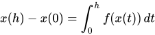
Unfortunately further approximations are needed, as the right hand side is still impossible to evaluate exactly. We look for a Runge–Kutta approximation for $x$ evaluated at these times. Let $x_{1}$ and $x_{2}$ be shorthands for these two quadrature points.

$x_{1}=x\left(\left({\frac {1}{2}}-{\frac {\sqrt {3}}{6}}\right)h\right)\approx x(0)+a_{11}k_{1}+a_{12}k_{2}.$

$x_{2}=x\left(\left({\frac {1}{2}}+{\frac {\sqrt {3}}{6}}\right)h\right)\approx x(0)+a_{21}k_{1}+a_{22}k_{2}.$

Here $k_{i}=f(x_{i})$ . This is an implicit constraint that must be solved by a root finding algorithm like Newton's method. The values of the Runge-Kutta parameters $a_{ij}$ can be determined from a Taylor series expansion in $h$ . The resulting scheme is the fourth order method.

A Practical Example

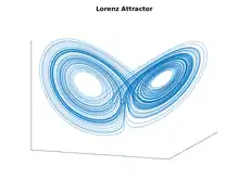
The Gauss-Legendre methods are implicit, so in general they cannot be applied exactly. Instead one makes an educated guess of $k_{i}$ , and then uses Newton's method to converge arbitrarily close to the true solution. Below is a Matlab function which implements the Gauss-Legendre method of order four.

%starting point
x = [ 10.5440; 4.1124; 35.8233];

dt = 0.01;
N=10000;
x_series = [x];
for i=1:N
  x = gauss_step( x, @lorenz_dynamics, dt, 1e-7, 1, 100);
  x_series = [x_series x];
end

plot3( x_series(1,:), x_series(2,:), x_series(3,:) );
set(gca,'xtick',[],'ytick',[],'ztick',[]);
title('Lorenz Attractor');
return;

function [td, j] = lorenz_dynamics(state)
  %return a time derivative and a Jacobian of that time derivative
  x = state(1);
  y = state(2);
  z = state(3);
  
  sigma = 10;
  beta  = 8/3;
  rho   = 28;
  
  td = [sigma*(y-x); x*(rho-z)-y; x*y-beta*z];

  j = [-sigma, sigma, 0;
        rho-z, -1, -x;
        y, x, -beta];
end

function x_next = gauss_step( x, dynamics, dt, threshold, damping, max_iterations )
  [d,~] = size(x);
  sq3 = sqrt(3);
  if damping > 1 || damping <= 0
    error('damping should be between 0 and 1.') 
  end
  
  %Use explicit Euler steps as initial guesses
  [k,~] = dynamics(x);
  x1_guess = x + (1/2-sq3/6)*dt*k;
  x2_guess = x + (1/2+sq3/6)*dt*k;
  [k1,~] = dynamics(x1_guess);
  [k2,~] = dynamics(x2_guess);
  
  a11 = 1/4;
  a12 = 1/4 - sq3/6;
  a21 = 1/4 + sq3/6;
  a22 = 1/4;
  
  error = @(k1,k2) [ k1 - dynamics(x+(a11*k1+a12*k2)*dt); k2 - dynamics(x+(a21*k1+a22*k2)*dt) ];
  er = error(k1,k2);
  iteration=1;
  while( norm(er) > threshold && iteration < max_iterations )
    fprintf('Newton iteration %d: error is %f.\n', iteration, norm(er) );
    iteration = iteration + 1;
    
    [~, j1] = dynamics(x+(a11*k1+a12*k2)*dt);
    [~, j2] = dynamics(x+(a21*k1+a22*k2)*dt);
    
    j = [ eye(d) - dt*a11*j1, -dt*a12*j1;
         -dt*a21*j2, eye(d) - dt*a22*j2 ];
     
    k_next = [k1;k2] - damping*linsolve(j,er);
    k1 = k_next(1:d);
    k2 = k_next(d+(1:d));
    
    er = error(k1,k2);
  end
  if norm(er) > threshold 
    error('Newton did not converge by %d iterations.', max_iterations); 
  end
  x_next = x + dt/2*(k1+k2);
end

This algorithm is surprisingly cheap. The error in $k_{i}$ can fall below $10^{-12}$ in as few as 2 Newton steps. The only extra work compared to explicit Runge-Kutta methods is the computation of the Jacobian.

An integrated orbit near the Lorenz attractor.

Notes

Iserles 1996, p. 47
Iserles 1996, p. 63
Iserles 1996, p. 47

References

Iserles, Arieh (1996), A First Course in the Numerical Analysis of Differential Equations, Cambridge University Press, ISBN 978-0-521-55655-2.

This article is issued from Wikipedia. The text is licensed under Creative Commons - Attribution - Sharealike. Additional terms may apply for the media files.

[1] Iserles 1996, p. 47

[2] Iserles 1996, p. 63

[3] Iserles 1996, p. 47