Tandem rolling mill
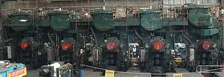
A Tandem rolling mill is a Rolling mill with 2 or more close-coupled Stands, each of which is setup for rolling by using its Spring Curve and the Compressive Curve of the metal so that both the Rolling Force and the exit thickness of each Stand are determined.
%252C_entry_bridle%252C_2_stands%252C_exit_bridle_and_coiler_(tension_reel).jpg.webp)
The main advantages of a Tandem Mill are: only one single pass is required which saves time and increases production; also greater tensions are possible between the stands, and this increases the reduction possible in the stands for the same roll force.
One disadvantage of a Tandem Mill is the high capital cost compared to that of a single stand Reversing Mill.
Note that, for Mills rolling thinner strip, Bridles may be added either at the entry and/or the exit to increase the strip tension near the adjacent stands further increasing their reduction capability.

This article describes the characteristics of a Mill Stand and the properties of a metal (especially steel) using both equations and diagrams.
Mill stand characteristics
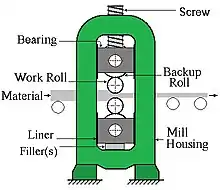

The Mill Stand spring curve is obtained by pressing the Work Rolls together with increasing force. This causes the Work Rolls to bend, the Screw-downs to compress and the Mill Housings to stretch. To reduce Work Roll bending, a much larger roll is positioned above the top Work Roll and another is placed below the bottom Work Roll. This arrangement is called a 4-high Mill.
The red line in Graph 2 is the linear approximation F = Fd – M * ( S – Sd )
or conversely, the Screw-down position S = Sd – ( F – Fd ) / M equation 1
where M is called the Mill modulus and is the slope of the spring curve in the area of the datum point (Sd, Fd). For most Mills M is approximately 4 MN/mm. Larger values would require much thicker Mill housings and Screw-downs.
Wood and Ivacheff[1] analysed the information obtained when measuring the Mill modulus by pressing the Work Rolls together until a typical rolling force was reached, and then they continued to measure the force and Screw-down position as the Rolls were lifted. The shape of the plotted figures (overlaid, looped, or a figure eight) was found to give good indication of the Mill Stand’s condition.
The datum point is chosen so that the Screw-down position S is never negative. This was necessary with the control computers of the 1960s, such as the GE/PAC 4020 installed at the then Australian Iron & Steel (now Bluescope Steel's Port Kembla) Plate Mill, which used assembler language that did not like negative numbers.
Also, a datum point is used rather than trying to measure the point at which the Force just becomes zero.
The exact equation used to calculate the required Screw-down setting for a required force is: -
- S = Sd + Sa – ( F – Fd ) * { 1 – k * log ( F/Fd ) } / M equation 2[2]
where: k is the value to best suit the measured values
- Sa is an adapter which corrects for the thermal expansion of the Mill Housing and Rolls as they warm up during rolling. It is set to zero after a Work Roll change (datum just performed with the new rolls at room temperature). Using the measured values of F and S during the rolling of one piece of metal, then Sa can be calculated for use at the start of the next piece.
Roll force measurement
To obtain the true roll force between the Work Rolls one must consider the position of the Load Cells that measure the force; are they with the Filler Plates under the bottom BU Roll bearings, or on top of the top BU Roll bearings.
Another thing that must be considered (if it is present) is Work Roll Balance.
The Work Roll balance cylinders act to separate the Work Rolls (no force between them) when the Screw-downs are raised; that is, the force of the balance cylinders Fbal is just greater than the weight of the top roll set, (Wtbu + Wtwr).
Balance OFF, load cells above top BU roll bearings
- With the Screws raised, they exert no force on the top BU Roll bearings. So the Load Cells output zero force, but the top rolls press down on the bottom Work Rolls; therefore the weight of the top roll set (Wtbu + Wtwr) must be added to the Load Cell reading.
Balance ON , load cells above top BU roll bearings
- With the Screws raised, the Load Cells have the top roll set pressed against them with a force of Fbal - (Wtbu + Wtwr) and this value must be subtracted from the Load Cell reading to obtain the actual force of zero.
Balance OFF, load cells under bottom BU roll bearings
- Again with the Screws raised, they exert no force on the top BU Roll bearings. However, the Load Cells have the weight of all four Rolls pressing down on them, and so their output is 2•Wtbu + 2•Wtwr But the true force on the bottom Work Roll is just the weight of the top roll set, so the weight of the bottom Work Roll and the bottom BU Roll (Wtbu + Wtwr) must be subtracted from the Load Cell reading.
Balance ON , load cells below bottom BU roll bearings
- The Load Cells have the weight of the bottom roll set pressed onto them by the Work Roll balance cylinders, so they read Fbal + (Wtbu + Wtwr). However, this must be subtracted to obtain the true roll force of zero.
- This was the condition of the Mill when Graph 2 was obtained. Note that, when the Work Roll balance was turned OFF, then Fbal became zero and so the correcting term was still correct.
The above Roll Weights Wtbu and Wtwr are only nominal values; the actual values will vary a little depending on how many times the Rolls have been ground down between campaigns.
Since the Roll Weights are only nominal values, any residual error should be slowly zeroed out whenever the roll balance is ON and the Screws are raised sufficiently.
Steel characteristics
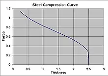
A useful formula for the compression curve of Steel is: -
- K = k0 + k1 { k2 + loge(H/h) }k3 equation 3[2]
where K is the metal’s hardness;
- H is the metal’s initial thickness;
- h is the metal’s exit thickness;
- k0 and k3 are grade dependent constants;
k0 moves the curve vertically, i.e. it sets the initial yield stress; k3 changes the slope, i.e. the metal’s work hardening rate.
The initial steep section is elastic compression. The effective height of this is reduced by the Entry and Exit Tensions when present, as in a Tandem Mill. Notice that the curve becomes steeper as the thickness approaches zero, i.e. it would take infinite force to make the steel infinitely thin.
The slope of the plastic region around the operating point is normally represented by the letter Q.
Mill setup calculation – a graphical solution
The term "Setup" is used for the calculation of the actuator settings required by each Mill Stand to roll the product. These settings include the initial Screw-down position, the main drive speed, and the entry and exit tension references where applicable.
This Setup calculation is normally performed either in a lower-level Computer or a PLC that controls a Rolling Mill Stand(s).
If the Mill Stand Spring curve and the Compression Curve for the Strip are drawn against the same distance axes, then the intersection point gives the solution of expected Rolling Force F, and final Strip Thickness h, and also the required initial Screw-down position So.
In its simplest form h = S – So – (F – Fo) / M equation 4
This equation is known as the BISRA equation. It is also known as the Gaugemeter equation because measurements of S and F can be used to calculate the exit thickness as measured by an instrument called a thickness gauge.
If the Work Rolls are initially pressed together by the Screw-downs, then there will be a force Fo acting between the top and bottom Work Rolls before the strip is present. In this situation, the Mill is said to be set "below face", as shown in Graph 1. This is often the case with thin strip.
However, if there is an actual gap before the metal enters the Mill, then Fo will be zero, and (from equation 1) So must be greater than Sd + Fd / M
The calculation can be repeated for any following Stands with the exit thickness h of the one Stand becoming the entry thickness H of the next Stand. Note that the Compression Curve will have a greater or lesser elastic region depending on the entry and exit tension stresses of that next Stand.
Associated rolling theory
Sensitivities and their uses
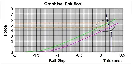
If during rolling, it is necessary to move the Screw-downs to correct either the Rolling Force or the exit Strip Thickness, then consider the triangle (shown circled in the Graph on the right) created when the Screw-downs are moved down from the purple to the green.
Note that the Strip becomes thinner and the Rolling Force increases.
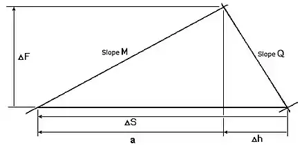
ΔS = Δh + a with ΔH = 0, but the slope Q = ΔF / Δh, and the slope M = ΔF / a
Therefore, ΔS = ΔF / Q + ΔF / M
Which gives, ΔS / ΔF = 1 / Q + 1 / M equation 5
This term is used to ensure the control of the rolling force using the Screws is independent of the metal being rolled.
Using ΔF = Q . Δh
Gives ΔS / Δh = 1 + Q / M equation 6
This factor is used to guarantee that the control of the exit thickness by the Screws is independent of the metal being rolled.
Forging and extrusion
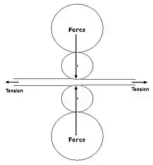
One could say the steel is compressed by the force of the Work Rolls, equivalent to forging; however, if there are tensions present, then it could be said that the steel is stretched by the tension pulling it through the rotating Work Rolls, as in extruding through a die.
The tension effect should be represented in Graphs 1 and 3 above, by drawing the Steel Compression Curve with the Elastic region reduced by an amount equal to the Tension induced strain.
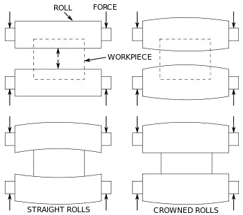
The relationship of the Rolling Force to the entry and exit Strip Tensions is important in determining the finished Strip Flatness.[3] Too much force produces strip with edge wave (often called "pressure wave"). Too much tension, that is too little force, can cause centre buckle (depending on the Crown of the Rolls).
The tension stress is 30% to 50% of the yield stress for Cold Mills and often higher in Hot Mills (which can result in heavy necking and even strip breaks).

Note that the force is offset from the Work Roll centres because the strip is thicker at the entry than at the exit; this is one component of the torque that the Main Drives must supply. The other component is the difference in the tension forces. If the exit tension force is much greater than the entry tension force, then the tension torque may be larger than the torque due to the rolling-force and the Main Drives will generate power.
The Neutral Point, or no-slip point[4] is the point within the roll bite where the Work Rolls and the Strip are doing the same speed.
The position of the Neutral Point is influenced by the entry and exit tensions.

Shudder occurs when the Neutral Point is at an edge of the Roll Bite; that is the Work Rolls are alternately grabbing the Strip and letting it slip.
Forward Slip (1+f) is the ratio of the Exit Strip Speed to the Work Rolls peripheral speed. Backward slip (1-b) is the ratio of the Entry Strip Speed to the Work Rolls peripheral speed
Back-up roll bearings speed effect
The Back-up Roll bearings are usually white-metal bearings which rely on a film of oil between the shaft and the white-metal to reduce the friction; see in Sketch 6.
As the speed increases more oil is dragged into the active region of the bearing and this increases the thickness of the oil film in this region. This pushes the top Work Roll down and the bottom Work Roll up, which reduces the roll gap in the same manner as running the Screws down. To compensate for this, most Screw-down control loops include a feedforward parameter derived from either; an equation of rolling speed, or a value extracted from a lookup table using interpolation.
To ensure an oil film exists even at zero speed; pumps are often used to force oil through very tiny holes into the bearing’s active region; this is referred to as hydrostatics.

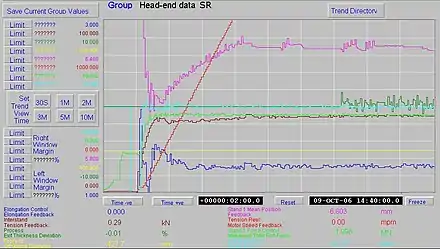
In Chart 1, the scale for the Screw-downs position (mauve trace) was 0.2 mm per division; this was too coarse. Consequently Chart 2 was created from a similar coil, but with a Screw-down position scale of 0.06 mm per division; that is, from 5.8 mm to 6.4 mm.
In the chart recordings, notice that the force (light green trace) has been held constant by the automatic control, which has raised the Screw-downs (mauve trace) as the speed (red trace) has increased. This increase in Screw position is a measure of the White Metal Bearing speed effect.
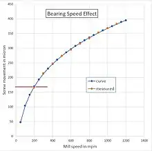
For a more accurate measurement, the force of each Mill Stand should be measured as it is run through its speed range without strip present.
The values measured from Chart 2 were plotted in an Excel spread-sheet. The equation that was used to match the measured points was 680*POWER((speed/1200),0.225)-285.
Note that the use of oil hydrostatics can hold the oil film nearly constant up to about 20% of full speed; hence no Screw-down movement would be required in that low speed range (this is shown as the red line in the graph of the measured points).
Now recall the Gaugemeter equation in its simplest form: -
- h = S – Sd – (F – Fd) / M
This equation must be modified to include the Backup Roll bearing speed effect Sv especially when rolling Product which has a thickness similar to the speed effect (~400 μm at some Temper Mills).
- thus h = S – Sd – Sv – (F – Fd) / M equation 7
Back-up roll eccentricity
Virtually all of the strip thickness variation is the result of the eccentricity and out-of-roundness of the Back-up Rolls from about Stand 3 of the Hot Strip Mill through to the Finished Product.

The Back-up Roll eccentricity can be up to 100 μm in magnitude per stack. The eccentricity can be measured off-line by plotting the force variation against time with the Mill on creep, no strip present, and the Mill Stand below face.
A modified Fourier analysis was employed by the 5 Stand Cold Mill at Bluescope Steel, Port Kembla from 1986 until that Cold Mill ceased production in 2009. Within each coil, the exit thickness deviation times 10 for every meter of strip was stored in a file. This file was analyzed separately for each frequency/wavelength from 5 m to 60 m in steps of 0.1 m. To improve the accuracy, care was taken to use a full multiple of each wavelength (100*). The calculate amplitudes were plotted against the wavelength, so that the spikes could be compared to the expected wavelengths created by the Backup Rolls of each Stand.
If a Mill Stand is fitted with Hydraulic Pistons in series with, or instead of the electrically driven Mechanical Screws, then it is possible to eliminate the effect of that Stands Back-up Roll eccentricity.[5][6] While rolling, the eccentricity of each Back-up Roll is determined by sampling the roll force and assigning it to the corresponding portion of each Back-up Roll’s rotational position. These recordings are then used to operate the Hydraulic Piston so as to neutralize the eccentricities.
Mass flow
A Rolling Mill does not create nor destroy steel during normal steady state rolling.
That is; the same mass of steel leaves the Mill as entered it.
And so; expressing the entry volume as H . Wn. ℓ, and the exit volume h . Wx . L
- But the entry length ℓ = v . t and the exit length L = V t where t is the total rolling time.
- Therefore ρ . H . Wn . v . t = ρ . h . Wx . V . t
The density ρ is unaffected by the rolling process and can be cancelled out. The width may change, but it does so by an insignificant amount (only a fraction of the strip thickness), and so the change may be ignored when rolling thin (< 1 mm) strip. The Roll Force tends to widen the strip, while the entry and exit tensions (when present) tend to make the strip narrower.

So, cancelling the density ρ, the width W, and the time t, gives
- h . V = H . v equation 8
This can be used in a Rolling Mill to calculate the exit thickness h that the X-ray gauge will measure when the corresponding portion of the Strip finally reaches the Gauge.
By assuming all of the Cold Mill head-end off-gauge has been completely removed by the previous Continuous Annealing Line; the scheduled entry thickness can be substituted in place of the actual entry thickness, H.[7] Then the Entry Bridle and Exit Bridle speeds can be used as the measurements of entry speed, v and exit speed, V respectively.
The resulting Calculated Thickness Deviation can be seen as the light blue trace in Chart Recording 3. Notice that the thickness control was working at thread speed (red trace). In the Block Diagram, the calculated gauge (thickness) is q62 and the thickness error is q66. Note the use of the Sensitivity Factor dS/dh as q2. There are two other interesting factors with this control: -

A bumpless PI control
Initially the control appears to be a PD control with q18 containing a P term equal to q16 times the gain q4, plus a D term being the constant q10 times the change in q16. However, since q20 is effectively added to itself, this summation converts the P term into an Integral, and the D term becomes a Proportional term. This arrangement has the advantage that the gains q4 and q10 can be changed while the control loop is active without causing a step in the output q20; that is, it’s a Bumpless control. The rate-of-change limit is designed to prevent the equivalent of integral windup.
An NIC trim into the inter-stand tension control
Normally moving the Screw-downs to correct the Strip Thickness would perturb the Inter-stand Tension; its control would then need to trim the speed of the appropriate Stand to restore the tension. So, what is required, is a compensating trim applied to the Tension Control at the same time as the Thickness trim goes to the Screw-downs. This is referred to as a Non-Interactive Control;[8] that is, the Thickness correction no-longer disturbs the Tension. In the Block Diagram, the Screw Trim q20 is converted into a compensating IS Tension trim using the sensitivity factor dT/dS (the value of this was measured by applying a small step change to the thickness reference and looking for any change in the IS Tension).
For the coil in Chart Recording 1 above, the Cold Mill Head-end off-gauge was not fully removed at the CA line; this can be seen as the difference between the X-ray Deviation (green trace) and the calculated thickness deviation (light blue trace).
Bridle rolls
Bridle Rolls are used to increase or decrease the strip tension in a Processing Line or Rolling Mill.
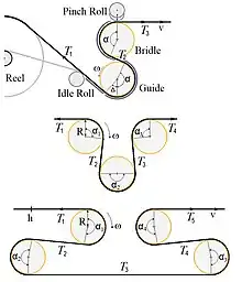
The Bridle Rolls normally come in a set of 2, 3, or 4 rolls of equal diameter, with each Roll individually powered by an electric motor/generator.[9] The drives of the Exit Bridle generate power as they decrease the Strip tension. This power is nearly equal to that used by the Entry Bridle to increase the Strip tension; the difference is just the mechanical and electrical losses.
To assist with threading there are normally Guides and even a Pinch Roll or Rolls, as shown for the 2 Roll Bridle in Sketch 7
To determine the size of the electrical drives, it is necessary to calculate the values of the intermediate tension or tensions.[10]
The maximum tension difference ΔT across a single Bridle Roll is determined by the wrap angle α (in radians) of the Strip around that Roll, and the roll-to-strip sliding friction μ, i.e. T2 = T1 • eμ•α.[9] equation B-1
The power required to drive such a Bridle is (T2 – T1) • (R + h/2) • ω i.e. (T2 – T1) • v
- where v is the strip speed in m/sec
- h is the strip thickness in meters
- R is the diameter of the Bridle Rolls in meters
- and ω is the Bridle’s angular speed in radians per second.
The electrical power required by the Drive Motor = Volts • Amps. The voltage can be regulated according to the strip speed, leaving the current to be proportional to the required tension change.
To prevent slippage, the Bridle Rolls within a set are operated at only a fraction p of the maximum tension difference, so the actual tension difference across each Bridle Roll will be ep•μ•α. That is, a lower value of friction is used in the calculations.
Consider the simplest case: -
A 2 Roll Bridle set with both Rolls having the same wrap angle α. Then T2 = T1 • e p•μ•α, and T3 = T2 • e p•μ•α.
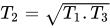
Therefore T2 / T1 = T3 / T2 which gives , T22 = T1 • T3
And so equation B-2
Now consider an example: -
- Let T3 = 2.0 • T1, then, T2 = 1.4142 • T1
- so the tension across the first Bridle will be ( 1.4142 – 1.0) • T1 = 0.4142 • T1
- and the Tension across the second Bridle will be ( 2.0 – 1.4142) • T1 = 0.5858 • T1
And so, the second Bridle requires just over 40 % more motor power compared to the first.
If one wishes to reduce the number of spares; then it is desirable to have motors of the same power.
To do that, the wrap angle on the first Bridle must be increased so that the tension difference across both Bridles is the same;
T3 - T2 = T2 - T1 That is T2 = 1.5 • T1 equation B-3
Let the wrap angle of Bridle Roll 1 be (α+Δ), where α is the wrap angle of Bridle Roll 2.
That is T2 / T1 = e p•μ•(α+Δ) = 1.5
Taking logarithms of both sides gives p•μ•(α+Δ) = lne(1.5) equation B-4
For Bridle Roll 2: T3 / T2 = e p•μ•α = 2.0 / 1.5
Again, taking logarithms gives p•μ•α = lne(1.3334) equation B-5
From equations B-4 and B-5: Δ = 0.4094 • α equation B-6
Now consider a 4 Roll Bridle with Tensions T1 through to T5. Normally in such a Bridle set all of the Rolls have the same Strip wrap angle, as shown in Sketch 7
The wrap angle from T1 to T3 is the same as that from T3 to T5.
Therefore, using equation B-2 equation B-7
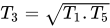
Similarly, equation B-8
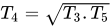
So if we let T5 = 4.0 • T1 then T3 = 2.0 • T1 which gives T2 = 1.4142 • T1
And finally = 2.8284 • equation B-9


Discontinuity in the stress verses strain of annealed steel
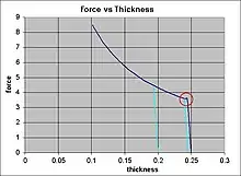
The discontinuity in the stress/strain of annealed steel[11] makes it impossible to create round tinned steel-cans. Wherever the steel bends first is where most of the bending will occur, rather than uniformly.
The discontinuity is shown within the red circle in Graph 6. It is the reason the Strip is given a light reduction (~1.3%) normally referred to as an elongation or extension.
Since it is referred to as an elongation and not a reduction, this Strip is said to have been reduced only once (at the Cold Mill prior to annealing); hence the term Single Reduced, SR.
After the elongation the discontinuity is no longer present.
Alternatively; after annealing, the steel strip can be reduced a second time (by up to 30%) to make it both thinner and work hardened. [12] When this is done, the strip is said to have been reduced twice; that is, Doubled Reduced, DR.
Inter-stand tension control
Consider a Violin String: -
- The Tension Force F established in the String of length ℓ is related to e, the amount the String is stretched: -
- ( F . ℓ ) / ( e . A ) = E equation 9
- Where F / A is Tension Stress (Tension force / unit area)
- e / ℓ is the Strain (amount of stretch, in PU)
- E is Young’s modulus of elasticity[11]
- Where F / A is Tension Stress (Tension force / unit area)
- and the area A is equal to the strings cross-sectional area.
Now consider the strip between the Stands of a multi-stand Mill: -
- In time Δt an extra length of ℓ = V.Δt leaves the previous Stand, where V is the strip’s exit speed.
- To establish the tension in this piece of strip, requires it to be stretched by an amount equal to F.V.Δt / ( E.A ) in the time interval of Δt; that is, a speed of F.V / E.A where the strip’s cross-sectional area A is equal to its width W times its thickness h,
- If the speed difference between the next stand’s entry and the previous stand’s exit is different to this, then the strip of length L between the two stands will stretch or relax according to the integral of speed difference, and this will change the actual tension as shown in the Block Diagram.
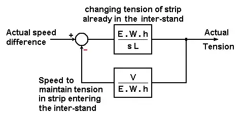

The overall transfer function from speed-difference to tension is: -
- E . W . h / (sL + V) equation 10
Therefore, the control loop must divide the tension error by the strip width W and the strip thickness h in order to have a consistent response.
In Chart Recording 4, the two components necessary to change the Tension (brown trace) can be seen in the Speed Trim (light blue trace). There is the extra speed difference necessary to stretch the Strip already in the Inter-stand Gap (large trim); and the slight increase in speed difference to maintain the new level of Tension.
Rolling mill definitions
Reduction
This definition only applies to the rolling of slabs, plates and strip in a Rolling Mill.
Reduction, r is defined as the per-unit change in thickness with respect to the entry thickness H, and so r = (H – h) / H where h is the exit thickness.[13][14]
Note that, as the material is reduced, its length becomes proportionately longer; this can be seen in the attached GIF movie above.
There are many other definitions of the word Reduction; such as in Chemistry, Medicine, Surgery, Safety, Investment, and in a more general sense, such as in cooking and waste reduction, etc.
If the required reduction is very small (< 2%) it is normally measured as elongation, e; which is defined as the per-unit increase in length with respect to the original length.
Given an entry length ℓ, then e = (L – ℓ) / ℓ where L is the final length.
.jpg.webp)
If the width is unaffected (as is the case when rolling thin strip <2mm), then the Mass Flow concept, gives H . ℓ = h . L
- Thus elongation, e = (H – h) / h
Note that the difference (H – h) is now with respect to the exit thickness h and not the entry thickness H; so, reduction and elongation are not exactly equal.
Elongation
When the reduction is small (< 2%), it is normally referred to as an elongation or an extension.
.jpg.webp)
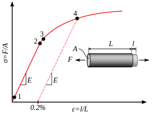
Elongation, e is defined as the per-unit increase in length due to a decrease in area with respect to the entry, regardless of shape (as shown for a round bar in Graph 7 to the right).
Given an entry length ℓ, then e = (L – ℓ) / ℓ where L is the final length.
If the width is unaffected (as is the case when rolling thin strip <2mm), then the Mass Flow concept, gives H . ℓ = h . L
- Thus elongation, e = (H – h) / h
When the elongation is large it is normally measured as reduction, r which is defined as the per-unit change in thickness with respect to the entry thickness H; and so if h is the exit thickness,[13][14]
- Reduction, r = (H – h) / H
These definitions apply to the rolling of thin strip in a Rolling Mill.
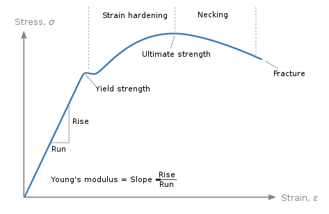
An elongation of typically 1.3% is performed to eliminate the discontinuity (seen at yield point in Graph 8) in the stress verses strain reaction of thin steel strip[15] before it is tinned ready for making cans intended for containing preserved foods.
There are many other definitions of the word Elongation; such as in Astronomy, Plasma physics, Biology (genetics), and in a more general sense, such as referring to the lengthening of an elastic band.
See also
References
- Wood, G.E.; Ivacheff, D.P. (January 1977). "Mill Modulus Variation and Hysteresis – Their Effects on Hot Strip Mill AGC". Iron and Steel Engineer: 65–71.
- Carlton, A.J.; Edwards, W.J.; Thomas, P.J. (March 1977). "Formulae for Cold Rolling Analysis". Proc. AIME Annual Meeting: 238–248.
- You, Changyu (2008). An Artificial Intelligence Model to Simulate Strip Flatness in a Tandem Cold Rolling Mill. School of Mechanical, Materials and Mechatronic Engineering (M.E.). University of Wollongong.
- DeGarmo, E. Paul (1962). Materials and Processes in Manufacturing (second ed.). New York: The Macmillan Company. p. 307.
- Ballyns, J. (1990). "Method and apparatus for the detection and correction of roll eccentricity in rolling mills". US Patent 4,910,985.
- Edwards, W.J.; Thomas, P.J.; Goodwin, G.C. (July 1987). "Roll Eccentricity Control for Strip Rolling Mills". IFAC Proceedings. 20 (5, part 2): 187–198.
- Cox, A. D. (March 2014). "Low speed thickness control for a temper mill". Australian Journal of Electrical & Electronics Engineering. 11 (1). doi:10.7158/E13-030.2014.11.1.
- Bryant, G.F.; Edwards, W.J.; Higham, J.D. (1973). "A Non-Interactive Control Structure". In Bryant, G.F. (ed.). Automation of Tandem Mills, Part 2. London: The Metals Society.
- Avontuur, A.P.J. (March 2017). Maintenance Optimisation of Process Rolls, with an application to electrolytic tinning lines. School of Industrial Engineering (M.E.). Eindhoven University of Technology. pp. 21–22.
- Magura, D.; et al. (August 2019). "Distribution of the Strip Tensions with Slip Control in Strip Processing Lines". Energies, Switzerland: 3–6.
- DeGarmo, E. Paul (1962). Materials and Processes in Manufacturing (second ed.). New York: The Macmillan Company. pp. 15–18.
- DeGarmo, E. Paul (1962). Materials and Processes in Manufacturing (second ed.). New York: The Macmillan Company. pp. 22–23.
- Dr. Amr Shehata Fayed, Faculty of Engineering, Zagazig University. "Bulk Deformation Forming Processes". Flat Rolling Analysis slide 8. Charles Palmer.CS1 maint: multiple names: authors list (link)
- Yuen, W.Y.D.; Dixon, A.; Nguyen, D.N. (1996). "The modelling of the mechanics of deformation in flat rolling". Journal of Materials Processing Technology. 60 (1–4): 87–94. doi:10.1016/0924-0136(96)02312-6.
- DeGarmo, E. Paul (1962). Materials and Processes in Manufacturing (second ed.). New York: The Macmillan Company. pp. 15–18.
Further reading
- Bland, D.R.; and Ford, H., "The calculation of roll force and torque in cold strip rolling with tensions", Proceedings of the Institute of Mechanical Engineers, vol 159, no. 1, 1948, pp 144-163.
- Sims, R.B., "The calculation of roll force and torque in hot rolling mills", Proceedings of the Institution of Mechanical Engineers, vol 168, no. 1, June 1954, pp 191-200.
- Lianis, G.; and Ford, H., "Control equations of multi-stand cold rolling mills", Proceedings of I.M.E., vol. 171, June 1957, pp 757-776.
- Bryant, G.F. (Editor); "Automation of Tandem Mills", The Iron & Steel Institute, London, 1973.
- Aeberli, K., "Combining the extended mass flow concept with eccentricity control for excellent gauge performance", Metals, Mining & More, Siemens, vol. 1, January 1997.
- Pittner, John; Simaan, Marwan A., "Tandem Cold Metal Rolling Mill Control using Practical Advanced Methods", Springer, London, 2010.