Lemniscate elliptic functions
In mathematics, the lemniscate elliptic functions are elliptic functions related to the arc length of the lemniscate of Bernoulli. They were first studied by Giulio Fagnano in 1718 and later by Leonhard Euler and Carl Friedrich Gauss, among others.

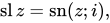
The lemniscate sine and lemniscate cosine functions, usually written with the symbols sl and cl (sometimes the symbols sinlem and coslem or sin lemn and cos lemn are used instead)[1] are analogous to the trigonometric functions sine and cosine. While the trigonometric sine relates the arc length to the chord length in a unit-diameter circle , the lemniscate sine relates the arc length to the chord length of a lemniscate


The lemniscate functions have periods related to a number 2.622057... called the lemniscate constant, the ratio of a lemniscate's perimeter to its diameter.

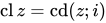
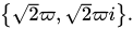
The sl and cl functions have a square period lattice (a multiple of the Gaussian integers) with fundamental periods [2] and are a special case of two Jacobi elliptic functions on that lattice, .

Similarly, the hyperbolic lemniscate functions slh and clh have a square period lattice with fundamental periods
The lemniscate functions and the hyperbolic lemniscate functions are related to the Weierstrass elliptic function .

Lemniscate sine and cosine functions
Definitions
The lemniscate functions sl and cl can be defined as the solution to the initial value problem:[3]

or equivalently as the inverses of an elliptic integral, the Schwarz–Christoffel map from the complex unit disk to a square with corners [4]

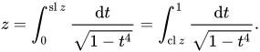
Beyond that square, the functions can be analytically continued to the whole complex plane by a series of reflections.
By comparison, the circular sine and cosine can be defined as the solution to the initial value problem:

or as inverses of a map from the upper half-plane to a half-infinite strip with real part between and positive imaginary part:


Arc length of Bernoulli's lemniscate


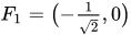
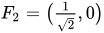
The lemniscate of Bernoulli with half-width 1 is the locus of points in the plane such that the product of their distances from the two focal points and is the constant . This is a quartic curve satisfying the polar equation or the Cartesian equation


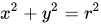
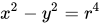
The points on the lemniscate at distance from the origin are the intersections of the circle and the hyperbola . The intersection in the positive quadrant has Cartesian coordinates:


Using this parametrization with for a quarter of the lemniscate, the arc length from the origin to a point is:[5]


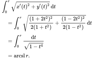
Likewise, the arc length from to is:

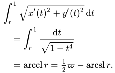
Or in the inverse direction, the lemniscate sine and cosine functions give the distance from the origin as functions of arc length from the origin and the point , respectively.
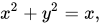
Analogously, the circular sine and cosine functions relate the chord length to the arc length for the unit diameter circle with polar equation or Cartesian equation using the same argument above but with the parametrization:


The lemniscate integral and lemniscate functions satisfy an argument duplication identity discovered by Fagnano in 1718:[6]

Later mathematicians generalized this result. Analogously to the constructible polygons in the circle, the lemniscate can be divided into n sections of equal arc length using straightedge and compass whenever n is of the form where k and m are non-negative integers and each pi (if any) is a distinct Fermat prime.[7] This was demonstrated by Niels Abel in 1827–1828.[8]

Arc length of rectangular elastica
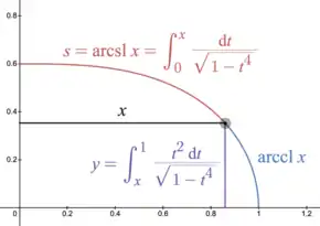
The inverse lemniscate sine also describes the arc length s relative to the x coordinate of the rectangular elastica.[9] This curve has y coordinate and arc length:

The rectangular elastica solves a problem posed by Jacob Bernoulli, in 1691, to describe the shape of an idealized flexible rod fixed in a vertical orientation at the bottom end and pulled down by a weight from the far end until it has been bent horizontal. Bernoulli's proposed solution established Euler–Bernoulli beam theory, further developed by Euler in the 18th century.
Lemniscate constant
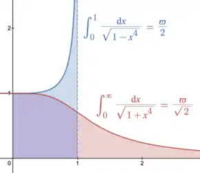
The lemniscate functions have minimal real period 2ϖ and fundamental complex periods and for a constant ϖ called the lemniscate constant,[10]


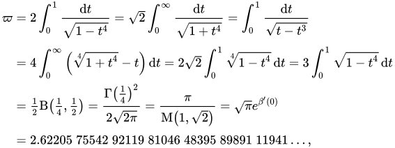
where Β is the beta function, Γ is the gamma function, M is the arithmetic–geometric mean and β is the Dirichlet beta function. The related constant is Gauss's constant. The lemniscate constant was proven transcendental by Theodor Schneider in 1937.[11] In 1975, Gregory Chudnovsky proved that π and ϖ are algebraically independent over .[12][13]


Geometrically, ϖ is the ratio of the perimeter of Bernoulli's lemniscate to its diameter. The lemniscate functions satisfy the basic relation

Furthermore, ϖ is related to the area under the curve . Defining , twice the area in the positive quadrant under the curve is In the quartic case,

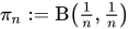


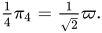
Euler discovered in 1738 that for the rectangular elastica:[14]

Viète's formula for π can be written:

An analogous formula for ϖ is:[15]

The Wallis product for π is:

An analogous formula for ϖ is:[16]

The ratio of these two is:

An infinite series for discovered by Gauss is:[17]


The Machin formula for π is and several similar formulas for π can be developed using trigonometric angle sum identities, e.g. Euler's formula . Analogous formulas can be developed for ϖ, including the following found by Gauss: [18]



In a spirit similar to that of the Basel problem,
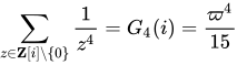
where are the Gaussian integers and is the Eisenstein series of weight .[19]


Symmetries
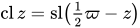
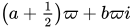
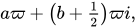
At translations of the lemniscate functions cl and sl are exchanged, and at translations of they are additionally rotated and reciprocated:


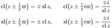
Doubling these to translations by a unit-Gaussian-integer multiple of (that is, or ), negates each function, an involution:


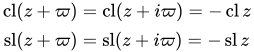
As a result, both functions are invariant under translation by an even-Gaussian-integer multiple of .[20] That is, a displacement with for integers a, b, and k.



This makes them elliptic functions (doubly periodic meromorphic functions in the complex plane) with a diagonal square period lattice of fundamental periods and .[21] Elliptic functions with a square period lattice are more symmetrical than arbitrary elliptic functions, following the symmetries of the square.
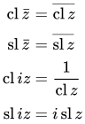
Reflections and quarter-turn rotations of lemniscate function arguments have simple expressions:
The sl function has simple zeros at Gaussian integer multiples of ϖ, complex numbers of the form for integers a and b. It has simple poles at Gaussian half-integer multiples of ϖ, complex numbers of the form , with residues . The cl function is reflected and offset from the sl function, . It has zeros for arguments and poles for arguments with residues




Pythagorean-like identity
_%253D_a(1_-_x%C2%B2y%C2%B2)_for_various_values_of_a.png.webp)
The lemniscate functions satisfy a Pythagorean-like identity:

As a result, the parametric equation parametrizes the quartic curve


This identity can alternately be rewritten:[22]


Defining a tangent-sum operator as gives:


Derivatives and integrals
The derivatives are as follows:
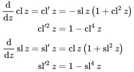
The second derivatives of lemniscate sine and lemniscate cosine are their negative duplicated cubes:
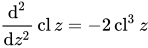
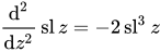
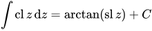
The lemniscate functions can be integrated using the inverse tangent function:

Argument sum and multiple identities
Like the trigonometric functions, the lemniscate functions satisfy argument sum and difference identities. The original identity used by Fagnano for bisection of the lemniscate was:[23]

The derivative and Pythagorean-like identities can be used to rework the identity used by Fagano in terms of sl and cl. Defining a tangent-sum operator and tangent-difference operator the argument sum and difference identities can be expressed as:[24]


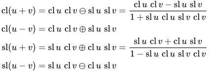
These resemble their trigonometric analogs:

Bisection formulas:
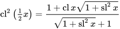
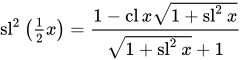
Duplication formulas:[25]
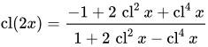
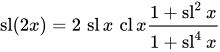
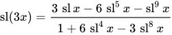
Triplication formulas:[25]

Specific values
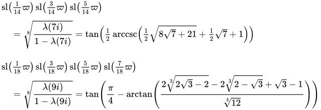
Just as for the trigonometric functions, values of the lemniscate functions can be computed for divisions of the lemniscate into n parts, using only basic arithmetic and square roots, whenever n is of the form where k and m are non-negative integers and each pi (if any) is a distinct Fermat prime.[26] However, the expressions become unwieldy as n grows. Below are the expressions for some n ≤ 10:














Power series
The power series expansion of the lemniscate sine at the origin is[27]

where the coefficients are determined as follows:



For example, to evaluate , it can be seen that there are only six compositions of that give a nonzero contribution to the sum: and , so





Relation to Weierstrass and Jacobi elliptic functions
The lemniscate functions are closely related to the Weierstrass elliptic function (the "lemniscatic case"), with invariants g2 = 1 and g3 = 0. This lattice has fundamental half periods and . The associated constants of the Weierstrass function are



The related case of a Weierstrass elliptic function with g2 = a, g3 = 0 may be handled by a scaling transformation. However, this may involve complex numbers. If it is desired to remain within real numbers, there are two cases to consider: a > 0 and a < 0. The period parallelogram is either a square or a rhombus. The Weierstrass elliptic function is called the "pseudolemniscatic case".[28] The square of the lemniscate sine can be represented as


where the second and third argument of denote the lattice invariants.

The lemniscate functions can also be written in terms of Jacobi elliptic functions. The Jacobi functions with positive real elliptic modulus have an "upright" rectangular lattice aligned with real and imaginary axes. Alternately, the Jacobi elliptic function with modulus i has a square period lattice rotated 1/8 turn.[29]


where the second arguments denote the elliptic modulus.
Relation to the modular lambda function
The lemniscate sine can be used for the computation of values of the modular lambda function:

For example:
Methods of computation
Several methods of computing involve first making the change of variables and then computing


A hyperbolic series method:[30]
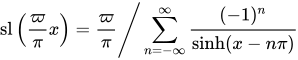
Fourier series method:[31]

The lemniscate sine can be computed more rapidly by
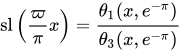
where
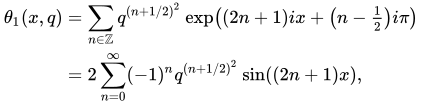

are the Jacobi theta functions.[32]
Another fast algorithm for computing is the following:[33]
- for each do
- if then
- for each n from N to 0 do
- return










This is effectively using the arithmetic-geometric mean and is based on Landen's transformations.[34]
Two other fast computation methods use the following sum and product series:




where

The following series identities were discovered by Ramanujan:[35]


Inverse functions
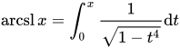
The inverse function of the lemniscate sine is the lemniscate arcsine, defined as:
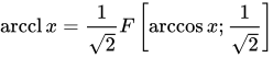
The inverse function of the lemniscate cosine is the lemniscate arccosine. This function is defined by following expression:

For x in the interval , and

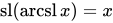
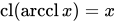
For the halving of the lemniscate arc length these formulas are valid:

Expression using elliptic integrals
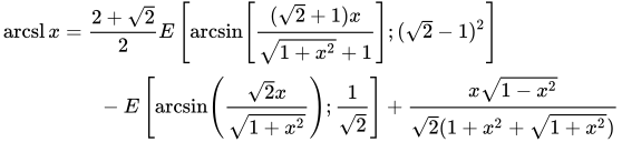
The lemniscate arcsine and the lemniscate arccosine can also be expressed by the Legendre-Form:
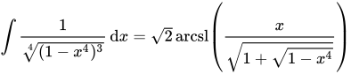
These functions can be displayed directly by using the incomplete elliptic integral of the first kind:


The arc lengths of the lemniscate can also be expressed by only using the arc lengths of ellipses (calculated by elliptic integrals of the second kind):
The lemniscate arccosine has this expression:
Use in integration
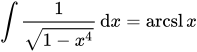
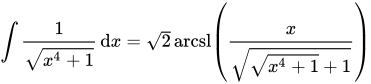
The lemniscate can be used to integrate many functions. Here is a list of important integrals (the constants of integration are omitted):








Hyperbolic lemniscate functions
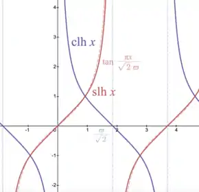
The hyperbolic lemniscate sine (slh) and cosine (clh) can be defined by their inverse functions as follows:

The complete integral has the value:

Therefore, the two defined functions have following relation to each other:
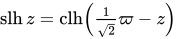
The product of hyperbolic lemniscate sine and hyperbolic lemniscate cosine is equal to one:

The hyperbolic lemniscate functions can be expressed in terms of lemniscate sine and lemniscate cosine:
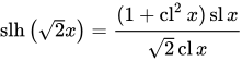
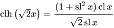
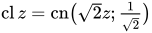
But there is also a relation to the Jacobi elliptic functions with the elliptic modulus one by square root of two:
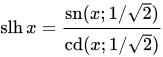
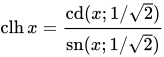
The hyperbolic lemniscate sine has following imaginary relation to the lemniscate sine:

This is analogous to the relationship between hyperbolic and trigonometric sine:
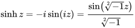
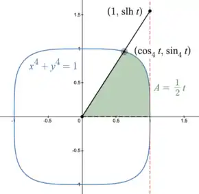
In a quartic Fermat curve (sometimes called a squircle) the hyperbolic lemniscate sine and cosine are analogous to the tangent and cotangent functions in a unit circle (the quadratic Fermat curve). If the origin and a point on the curve are connected to each other by a line L, the hyperbolic lemniscate sine of twice the enclosed area between this line and the x-axis is the y-coordinate of the intersection of L with the line .[36]


The hyperbolic lemniscate sine satisfies the argument addition identity:

The derivative can be expressed in this way:
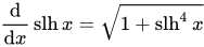
Furthermore the function is called Hyperbolic Lemniscate Tangent and the function is called Hyperbolic Lemniscate Cotangent.




Number theory
In algebraic number theory, every abelian extension of the Gaussian rationals is obtained by adjoining , where is a root of the equation and is a Gaussian integer.[37] This is analogous to the Kronecker–Weber theorem for the rational numbers which is based on division of the circle. Both are special cases of Kronecker's Jugendtraum, which became Hilbert's twelfth problem.


World map projections
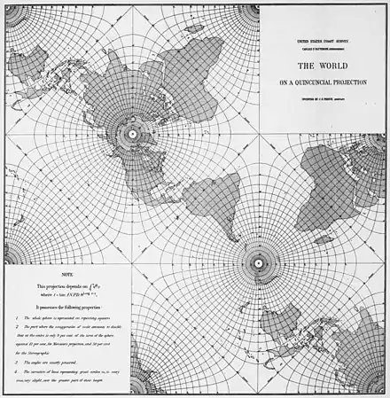
The Peirce quincuncial projection, designed by Charles Sanders Peirce of the US Coast Survey in the 1870s, is a world map projection based on the inverse lemniscate sine of stereographically projected points (treated as complex numbers).[38]
When lines of constant real or imaginary part are projected onto the complex plane via the hyperbolic lemniscate sine, and thence stereographically projected onto the sphere (see Riemann sphere), the resulting curves are spherical conics, the spherical analog of planar ellipses and hyperbolas.[39] Thus the lemniscate functions (and more generally, the Jacobi elliptic functions) provide a parametrization for spherical conics.
A conformal map projection from the globe onto the 6 square faces of a cube can also be defined using the lemniscate functions.[40] Because many partial differential equations can be effectively solved by conformal mapping, this map from sphere to cube is convenient for atmospheric modeling.[41]
See also
External links
- Parker, Matt (2021). "What is the area of a Squircle?". Stand-up Maths. YouTube.
Notes
- Gauss used the symbols sl and cl for the lemniscate sine and cosine, respectively. Ayoub (1984) uses sinlem and coslem. Whittaker and Watson (1920) use the symbols sin lemn and cos lemn. Some sources use the generic letters s and c. Prasolov & Solovyev (1997) use the letter φ for the lemniscate sine and φ′ for its derivative.
- and have the smallest absolute value of all periods whose real part is non-negative.
- Robinson (2019a) starts from this definition and thence derives other properties of the lemniscate functions.
- This map was the first ever picture of a Schwarz–Christoffel mapping, in Schwarz (1869) p. 113.
- Euler (1761), Siegel (1969). Prasolov & Solovyev (1997) use the polar-coordinate representation of the Lemniscate to derive differential arc length, but the result is the same.
- Siegel (1969), Schappacher (1997)
- Such numbers are OEIS sequence A003401.
- Abel (1827–1828), Rosen (1981), Prasolov & Solovyev (1997)
- Euler (1786), Sridharan (2004), Levien (2008)
- Schappacher (1997). OEIS sequence A062539 lists the lemniscate constant's decimal digits.
- Schneider (1937)
- G. V. Choodnovsky: Algebraic independence of constants connected with the functions of analysis, Notices of the AMS 22, 1975, p. A-486
- G. V. Chudnovsky: Contributions to The Theory of Transcendental Numbers, American Mathematical Society, 1984, p. 6
- Levien (2008). Todd (1975) calls these two factors and the lemniscate constants, and discusses methods for computing them.
- Levin (2006)
- Hyde (2014) proves the validity of a more general Wallis-like formula for clover curves; here the special case of the lemniscate is slightly transformed, for clarity.
- Bottazzini & Gray (2013), p. 60
- Todd (1975)
- Berndt, Bruce C. (1994). Ramanujan's Notebooks Part IV (First ed.). Springer Science+Business Media New York. ISBN 978-1-4612-6932-8. p. 249, 250
- The even Gaussian integers are the residue class of 0, modulo 1 + i, the black squares on a checkerboard.
- Prasolov & Solovyev (1997), Robinson (2019a)
- Lindqvist & Peetre (2001) generalizes the first of these forms.
- Ayoub (1984), Prasolov & Solovyev (1997)
- Euler (1761), §44 p. 79, §47 pp. 80–81
- Euler (1761) §46 p. 80
- Rosen (1981)
- "A104203". The On-Line Encyclopedia of Integer Sequences.
- Robinson (2019a)
- The identity can be found in Greenhill (1892), p. 33.
- Vigren & Dieckmann (2020), p. 7
- Reinhardt & Walker (2010), 22.11
- Reinhardt & Walker (2010), 22.2.E7
- Reinhardt & Walker (2010), §22.20(ii)
- Carlson (2010), §19.8
- Berndt, Bruce C. (1994). Ramanujan's Notebooks Part IV (First ed.). Springer Science+Business Media New York. ISBN 978-1-4612-6932-8. p. 247, 248, 253
- Levin (2006), Robinson (2019b)
- Ogawa (2005)
- Peirce (1879). Guyou (1887) and Adams (1925) introduced transverse and oblique aspects of the same projection, respectively. Also see Lee (1976). These authors write their projection formulas in terms of Jacobi elliptic functions, with a square lattice.
- Adams (1925)
- Adams (1925), Lee (1976).
- Rančić, Purser, & Mesinger (1996); McGregor (2005).


References
- Abel, Niels Henrik (1827–1828). "Recherches sur les fonctions elliptiques" [Research on elliptical functions]. Crelle's Journal (in French). 1827 (2): 101–181. doi:10.1515/crll.1827.2.101. "Recherches sur les fonctions elliptiques". Crelle's Journal. 1828 (3): 160–190. doi:10.1515/crll.1828.3.160.
- Adams, Oscar Sherman (1925). Elliptic functions applied to conformal world maps (PDF). US Government Printing Office.
- Ayoub, Raymond (1984). "The Lemniscate and Fagnano's Contributions to Elliptic Integrals". Archive for History of Exact Sciences. 29 (2): 131–149. JSTOR 41133708.
- Bottazzini, Umberto; Gray, Jeremy (2013). Hidden Harmony – Geometric Fantasies: The Rise of Complex Function Theory. Springer. doi:10.1007/978-1-4614-5725-1.
- Carlson, Billie C. (2010), "Elliptic Integrals", in Olver, Frank W. J.; et al. (eds.), NIST Handbook of Mathematical Functions, Cambridge University Press, ISBN 978-0-521-19225-5, MR 2723248
- Cox, David Archibald (2012). "The Lemniscate". Galois Theory. Wiley. pp. 463–514. doi:10.1002/9781118218457.ch15. ISBN 978-1-118-21845-7.
- Cox, David Archibald; Hyde, Trevor (2014). "The Galois theory of the lemniscate" (PDF). Journal of Number Theory. 135: 43–59. arXiv:1208.2653. doi:10.1016/j.jnt.2013.08.006.
- Enneper, Alfred (1890) [1st ed. 1876]. "Note III: Historische Notizen über geometrische Anwendungen elliptischer Integrale." [Historical notes on geometric applications of elliptic integrals]. Elliptische Functionen, Theorie und Geschichte (in German). Nebert. pp. 524–547.
- Euler, Leonhard (1761). "Observationes de comparatione arcuum curvarum irrectificibilium" [Observations on the comparison of arcs of irrectifiable curves]. Novi Commentarii Academiae Scientiarum Imperialis Petropolitanae (in Latin). 6: 58–84. E252. (Figures)
- Euler, Leonhard (1786). "De miris proprietatibus curvae elasticae sub aequatione contentae" [On the amazing properties of elastic curves contained in equation ]. Acta Academiae Scientiarum Imperialis Petropolitanae (in Latin). 1782 (2): 34–61. E605.
- Fagnano, Giulio Carlo (1718–1723). "Metodo per misurare la lemniscata" [Method for measuring the lemniscate]. Giornale de' letterati d'Italia (in Italian). 29: 258–269. "Giunte al primo schediasma sopra la Lemniscata". Giornale de' letterati d'Italia. 34: 197–207. "Metodo per misurare la lemniscata, schediasma II". Giornale de' letterati d'Italia. 30: 87–111. Reprinted in Fagnano (1911) [1850]. Opere Matematiche, vol. 2. Allerighi e Segati. papers 32, 33, and 34, pp. 293–313. (Figures)
- Greenhill, Alfred George (1892). The Applications of Elliptic Functions. MacMillan.
- Guyou, Émile (1887). "Nouveau système de projection de la sphère: Généralisation de la projection de Mercator" [New system of projection of the sphere]. Annales Hydrographiques, Ser. 2 (in French). 9: 16–35.
- Houzel, Christian (1978). "Fonctions elliptiques et intégrales abéliennes" [Elliptic functions and Abelian integrals]. In Dieudonné, Jean (ed.). Abrégé d'histoire des mathématiques, 1700–1900. II (in French). Hermann. pp. 1–113.
- Hyde, Trevor (2014). "A Wallis product on clovers" (PDF). The American Mathematical Monthly. 121 (3): 237–243. doi:10.4169/amer.math.monthly.121.03.237.
- Kubota, Tomio (1964). "Some arithmetical applications of an elliptic function". Crelle's Journal. 1964 (214/215): 141–145. doi:10.1515/crll.1964.214-215.141.
- Langer, Joel C.; Singer, David A. (2010). "Reflections on the Lemniscate of Bernoulli: The Forty-Eight Faces of a Mathematical Gem" (PDF). Milan Journal of Mathematics. 78 (2): 643–682. doi:10.1007/s00032-010-0124-5.
- Langer, Joel C.; Singer, David A. (2011). "The lemniscatic chessboard". Forum Geometricorum. 11: 183–199.
- Lawden, Derek Frank (1989). Elliptic Functions and Applications. Springer-Verlag. doi:10.1007/978-1-4757-3980-0.
- Lee, Laurence Patrick (1976). Conformal Projections Based on Elliptic Functions. Cartographica Monograph. 16. University of Toronto Press.
- Levien, Raph (2008). The elastica: a mathematical history (PDF) (Technical report). University of California at Berkeley. UCB/EECS-2008-103.
- Levin, Aaron (2006). "A Geometric Interpretation of an Infinite Product for the Lemniscate Constant". The American Mathematical Monthly. 113 (6): 510–520. JSTOR 27641976.
- Lindqvist, Peter; Peetre, Jaak (2001). "Two Remarkable Identities, Called Twos, for Inverses to Some Abelian Integrals" (PDF). The American Mathematical Monthly. 108 (5): 403–410. JSTOR 2695794.
- Markushevich, Aleksei Ivanovich (1966). The Remarkable Sine Functions. Elsevier.
- Markushevich, Aleksei Ivanovich (1992). Introduction to the Classical Theory of Abelian Functions. American Mathematical Society. doi:10.1090/mmono/096.
- McGregor, John L. (2005). C-CAM: Geometric Aspects and Dynamical Formulation (Technical report). CSIRO Atmospheric Research. 70.
- McKean, Henry; Moll, Victor (1999). Elliptic Curves: Function Theory, Geometry, Arithmetic. Cambridge. ISBN 9780521582285.
- Milne-Thomson, Louis Melville (1964). "16. Jacobian Elliptic Functions and Theta Functions". In Abramowitz, Milton; Stegun, Irene Ann (eds.). Handbook of Mathematical Functions. National Bureau of Standards. pp. 567–585.
- Neuman, Edward (2007). "On Gauss lemniscate functions and lemniscatic mean" (PDF). Mathematica Pannonica. 18 (1): 77–94.
- Nishimura, Ryo (2015). "New properties of the lemniscate function and its transformation". Journal of Mathematical Analysis and Applications. 427 (1): 460–468.
- Ogawa, Takuma (2005). "Similarities between the trigonometric function and the lemniscate function from arithmetic view point". Tsukuba Journal of Mathematics. 29 (1).
- Peirce, Charles Sanders (1879). "A Quincuncial Projection of the Sphere". American Journal of Mathematics. 2 (4): 394–397.
- Popescu-Pampu, Patrick (2016). What is the Genus?. Springer. doi:10.1007/978-3-319-42312-8.
- Prasolov, Viktor; Solovyev, Yuri (1997). "4. Abel's Theorem on Division of Lemniscate". Elliptic functions and elliptic integrals. American Mathematical Society. doi:10.1090/mmono/170.
- Rančić, Miodrag; Purser, R. James; Mesinger, Fedor (1996). "A global shallow-water model using an expanded spherical cube: Gnomonic versus conformal coordinates". Quarterly Journal of the Royal Meteorological Society. 122 (532): 959–982. doi:10.1002/qj.49712253209.
- Reinhardt, William P.; Walker, Peter L. (2010), "22. Jacobian Elliptic Functions", in Olver, Frank W. J.; et al. (eds.), NIST Handbook of Mathematical Functions, Cambridge University Press, ISBN 978-0-521-19225-5, MR 2723248
- Reinhardt, William P.; Walker, Peter L. (2010), "23. Weierstrass Elliptic and Modular Functions", in Olver, Frank W. J.; et al. (eds.), NIST Handbook of Mathematical Functions, Cambridge University Press, ISBN 978-0-521-19225-5, MR 2723248
- Robinson, Paul L. (2019a). "The Lemniscatic Functions". arXiv:1902.08614. Cite journal requires
|journal=(help) - Robinson, Paul L. (2019b). "The Elliptic Functions in a First-Order System". arXiv:1903.07147. Cite journal requires
|journal=(help) - Rosen, Michael (1981). "Abel's Theorem on the Lemniscate". The American Mathematical Monthly. 88 (6): 387–395. JSTOR 2321821.
- Schappacher, Norbert (1997). "Some milestones of lemniscatomy" (PDF). In Sertöz, S. (ed.). Algebraic Geometry (Proceedings of Bilkent Summer School, August 7–19, 1995, Ankara, Turkey). Marcel Dekker. pp. 257–290.
- Schneider, Theodor (1937). "Arithmetische Untersuchungen elliptischer Integrale" [Arithmetic investigations of elliptic integrals]. Mathematische Annalen (in German). 113 (1): 1–13. doi:10.1007/BF01571618.
- Schwarz, Hermann Amandus (1869). "Ueber einige Abbildungsaufgaben" [About some mapping problems]. Crelle's Journal (in German). 70: 105–120. doi:10.1515/crll.1869.70.105.
- Siegel, Carl Ludwig (1969). "1. Elliptic Functions". Topics in Complex Function Theory, Vol. I. Wiley-Interscience. pp. 1–89. ISBN 0-471-60844-0. MR 0257326.
- Snape, Jamie (2004). "Bernoulli's Lemniscate". Applications of Elliptic Functions in Classical and Algebraic Geometry (Thesis). University of Durham. pp. 50–56.
- Southard, Thomas H. (1964). "18. Weierstrass Elliptic and Related Functions". In Abramowitz, Milton; Stegun, Irene Ann (eds.). Handbook of Mathematical Functions. National Bureau of Standards. pp. 627–683.
- Sridharan, Ramaiyengar (2004). "Physics to mathematics: from lintearia to lemniscate – I" (PDF). Resonance. 9 (4): 21–29. "From lintearia to lemniscate II: Gauss and Landen's Work" (PDF). Resonance. 9 (6): 11–20.
- Todd, John (1975). "The lemniscate constants". Communications of the ACM. 18 (1): 14–19. doi:10.1145/360569.360580.
- Vigren, Erik; Dieckmann, Andreas (21 June 2020). "Simple Solutions of Lattice Sums for Electric Fields Due to Infinitely Many Parallel Line Charges". Symmetry. 12 (6): 1040.
- Whittaker, Edmund Taylor; Watson, George Neville (1920) [1st ed. 1902]. "22.8 The lemniscate functions". A Course of Modern Analysis (3rd ed.). Cambridge. pp. 524–528.
